Nitinol & Memory Alloys: Coding Soft Robotics Simulations

1. Introduction: The Rigid Body Limitation

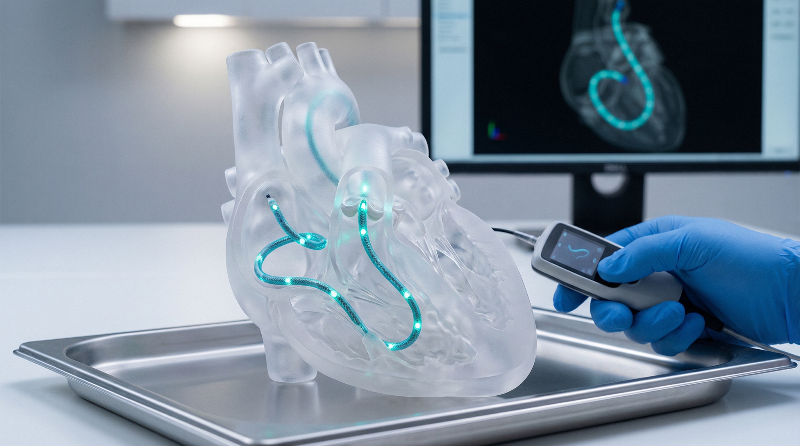
Imagine you are an engineer tasked with designing a surgical endoscope. It needs to navigate the tortuous geometry of the human vascular system, reaching deep into the cerebral arteries to treat an aneurysm. Traditional robotics, built on the foundation of rigid links and discrete joints actuated by bulky DC motors, fails here. The mechanics are too stiff, the footprint too large, and the risk of tissue damage too high. You need something that behaves less like a machine and more like organic muscle—compliant, continuous, and scalable.

Enter Soft Robotics, and specifically, the use of Shape Memory Alloys (SMAs) like Nitinol (Nickel-Titanium).

Nitinol is not merely a metal; it is a material that remembers. Through a complex interplay of thermal and mechanical energy, it can undergo large reversible deformations (Superelasticity) or recover a predefined shape upon heating (Shape Memory Effect). For a physicist, it is a fascinating thermodynamic engine. For a roboticist, it is the holy grail of actuation: high power-to-weight ratio, silent operation, and extreme compactness.

However, integrating Nitinol into a control loop is notoriously difficult. Unlike a standard servo where a PWM signal maps linearly to an angle, SMAs exhibit non-linear hysteresis, phase-dependent stiffness, and complex thermal dynamics. You cannot simply PID control an SMA without understanding the underlying physics.

In this post, we will bridge the gap between material science and software engineering. We will dissect the crystallographic phase transitions that drive Nitinol, derive the constitutive equations necessary for modeling, and finally, write a robust Python simulation engine to predict the behavior of an SMA actuator under thermal cycling. This is not just about writing code; it is about simulating reality to build better robots.

2. Theoretical Foundation: The Physics of Hysteresis

To simulate Nitinol, one must understand that it is a polymorphic material. It exists in two primary solid phases depending on temperature and stress:

Austenite (A): The high-temperature phase. It has a cubic crystal structure (highly symmetric) and is generally stiff (high Young's Modulus).
Martensite (M): The low-temperature phase. It has a monoclinic or tetragonal structure (low symmetry). It is softer and can exist in two forms: Twinned (self-accommodated) and Detwinned (reoriented by stress).

The Transformation Cycle

The magic happens during the phase transition. When you cool Austenite, it transforms into Twinned Martensite. There is no macroscopic shape change here, but the atomic lattice shears. If you apply stress to this Twinned Martensite, you "detwin" it, causing macroscopic strain (deformation). When you heat this Detwinned Martensite, the lattice springs back to the symmetric Cubic Austenite form, recovering the original shape with significant force. This is the Shape Memory Effect (SME).

Mathematical Modeling: The Constitutive Law

Simulating this requires a phenomenological constitutive model. The most widely used in engineering is the Brinson Model or variations of the Tanaka Model. We describe the stress ( $\sigma$ ) as a function of strain ( $\epsilon$ ), temperature ( $T$ ), and the martensite volume fraction ( $\xi$ ).

The fundamental constitutive equation is:

$\sigma - \sigma_0 = E(\xi)(\epsilon - \epsilon_0) + \Omega(\xi)(\xi - \xi_0) + \Theta(\xi)(T - T_0)$

Where:

$E(\xi)$ is the Young's Modulus (variable depending on phase).
$\Omega(\xi)$ is the Phase Transformation Tensor (relates strain to phase change).
$\Theta(\xi)$ is the Thermal Expansion Coefficient (often ignored in simple actuation models as phase strain dominates).
$\xi$ (Xi) represents the fraction of the material that is Martensite ( $0 \le \xi \le 1$ ).

The complexity lies in calculating $\xi$ . It is not a simple function of Temperature; it depends on the history of the material (Hysteresis). We define four critical temperatures:

$M_s, M_f$ : Martensite Start and Finish temperatures (Cooling).
$A_s, A_f$ : Austenite Start and Finish temperatures (Heating).

Typically, $M_f < M_s < A_s < A_f$ . The path from Austenite to Martensite follows a different curve than Martensite to Austenite, creating a hysteresis loop that represents energy dissipation. To code this, we use conditional kinetics functions, usually based on cosine or exponential distributions, to determine the rate of phase change $\dot{\xi}$ .

3. Implementation Deep Dive: Simulating the Actuator

We will implement a 1D simulation of a Nitinol wire lifting a static load. We will simulate the Shape Memory Effect by cycling the temperature (simulating Joule heating and convective cooling) and observing the strain recovery.

Prerequisites

We will use numpy for vector math and matplotlib for visualization. This simulation implements a simplified version of the Brinson model logic, focusing on the thermal-induced strain recovery.

Code Snippet 1: Material Class and Initialization

First, we define our NitinolActuator class with standard physical properties for a commercial NiTi wire.

import numpy as np
import matplotlib.pyplot as plt

class NitinolActuator:
    def __init__(self):
        # --- Material Constants ---
        # Transformation Temperatures (Celsius)
        self.M_f = 20.0  # Martensite Finish
        self.M_s = 40.0  # Martensite Start
        self.A_s = 50.0  # Austenite Start
        self.A_f = 70.0  # Austenite Finish
        
        # Moduli of Elasticity (GPa -> MPa for calculation)
        self.E_a = 70000.0  # Austenite Modulus
        self.E_m = 28000.0  # Martensite Modulus
        
        # Transformation Strain Limit (The max shape recovery)
        self.epsilon_L = 0.04  # 4% recoverable strain
        
        # Stress influence coefficients (simplified Clapeyron slopes)
        # How much transition temps shift with stress (MPa/C)
        self.C_m = 8.0 
        self.C_a = 13.8
        
        # --- State Variables ---
        self.xi = 1.0       # Initial Martensite fraction (1.0 = 100% Martensite)
        self.strain = 0.0   # Current strain
        self.stress = 0.0   # Current stress (MPa)
        self.T = 25.0       # Current Temperature (C)

    def get_modulus(self, xi):
        """Rule of mixtures for composite modulus."""
        return self.E_a + xi * (self.E_m - self.E_a)

Code Snippet 2: The Phase Kinetics (The Core Logic)

This is the most critical part. We must determine the Martensite fraction $\xi$ based on the current temperature and stress. Note that stress shifts the transition temperatures (This is why SMAs are stronger when hot).

    def update_phase_fraction(self, T_new, stress_new, dt):
        """
        Updates the martensite fraction (xi) based on temp and stress.
        Using a simplified cosine kinetic model.
        """
        # Calculate stress-adjusted transition temperatures
        # M_s_sigma = M_s + sigma / C_m
        Ms_sig = self.M_s + stress_new / self.C_m
        Mf_sig = self.M_f + stress_new / self.C_m
        As_sig = self.A_s + stress_new / self.C_a
        Af_sig = self.A_f + stress_new / self.C_a

        current_xi = self.xi
        
        # Determine Heating or Cooling based on Temperature derivative
        # In a real step, we compare T_new to self.T
        is_heating = T_new > self.T

        if is_heating:
            # Austenite Transformation (M -> A)
            if T_new > As_sig:
                if T_new >= Af_sig:
                    new_xi = 0.0
                else:
                    # Cosine interpolation between As and Af
                    # This creates the smooth curve of the hysteresis
                    arg = np.pi * (T_new - As_sig) / (Af_sig - As_sig)
                    # We scale based on previous history to allow partial loops
                    xi_source = 1.0 # Simplified: assuming full transformation cycle
                    new_xi = (xi_source / 2.0) * (np.cos(arg) + 1)
            else:
                new_xi = current_xi # No change yet
        
        else: # Cooling
            # Martensite Transformation (A -> M)
            if T_new < Ms_sig:
                if T_new <= Mf_sig:
                    new_xi = 1.0
                else:
                    # Cosine interpolation between Ms and Mf
                    arg = np.pi * (Ms_sig - T_new) / (Ms_sig - Mf_sig)
                    new_xi = (1.0 - (1.0/2.0) * (np.cos(arg) + 1))
            else:
                new_xi = current_xi

    return new_xi


### Code Snippet 3: Constitutive Update & Simulation Loop

Now we tie it together. We apply a constant stress (like a weight hanging on the wire) and cycle the temperature.

```python
    def solve_strain(self, xi, stress):
        """
        Inverted constitutive equation to find strain given stress and phase.
        Sigma = E(xi) * epsilon + Omega(xi)*xi ...
        Simplified for actuation: Strain is dominated by phase transformation.
        epsilon = stress / E(xi) + epsilon_L * xi
        """
        E = self.get_modulus(xi)
        # Transformation strain component + Elastic component
        elastic_strain = stress / E
        transformation_strain = self.epsilon_L * xi
        return elastic_strain + transformation_strain

# --- Simulation Setup ---
actuator = NitinolActuator()

# Simulation Parameters
time_steps = 200
temp_cycle = np.concatenate([
    np.linspace(25, 100, 100),  # Heating phase
    np.linspace(100, 25, 100)   # Cooling phase
])
constant_stress = 150.0  # MPa

history_strain = []
history_temp = []
history_xi = []

# --- Main Loop ---
for T_step in temp_cycle:
    # 1. Update Phase based on new Temp and Stress
    new_xi = actuator.update_phase_fraction(T_step, constant_stress, 0.1)
    
    # 2. Update Actuator State
    actuator.xi = new_xi
    actuator.T = T_step
    actuator.stress = constant_stress
    
    # 3. Calculate Resulting Strain
    current_strain = actuator.solve_strain(new_xi, constant_stress)
    actuator.strain = current_strain
    
    # 4. Data Logging
    history_strain.append(current_strain)
    history_temp.append(T_step)
    history_xi.append(new_xi)

# --- Visualization ---
plt.figure(figsize=(10, 6))
plt.plot(history_temp, np.array(history_strain) * 100, linewidth=2.5, color='firebrick')
plt.title('Nitinol Actuator Hysteresis: Strain vs Temperature (Constant Load)', fontsize=14)
plt.xlabel('Temperature (°C)', fontsize=12)
plt.ylabel('Strain (%)', fontsize=12)
plt.grid(True, linestyle='--', alpha=0.7)
plt.axvline(x=actuator.A_s + constant_stress/actuator.C_a, color='k', linestyle=':', label='As (stress adj)')
plt.axvline(x=actuator.M_s + constant_stress/actuator.C_m, color='b', linestyle=':', label='Ms (stress adj)')
plt.legend()
plt.show()

Explanation of Results

When you run this code, you will observe a distinct hysteresis loop.

Heating: As temperature rises past $A_s$ , strain decreases rapidly. The wire is contracting (actuating) as it reverts to the Austenite parent shape.
Cooling: As temperature drops, the wire remains contracted until it hits $M_s$ . Then, the modulus drops, and the internal phase transformation strain returns, causing the wire to elongate back to its "stretched" state under the load.

The width of this loop represents the thermal buffer inherent in the material. This is crucial for control systems; the wire does not contract and relax at the same temperature.

4. Advanced Techniques & Optimization

While the code above provides a solid kinematic foundation, applying this to high-performance soft robotics requires addressing several complexities.

1. Thermal Inertia and Heat Transfer

In the simulation above, we assumed we control temperature directly ( $T$ ). In reality, we control Current ( $I$ ) via Joule heating. The temperature evolution is governed by the heat balance equation:

$\rho V C_p \frac{dT}{dt} = I^2 R - h A (T - T_{amb})$

Where $h$ is the convection coefficient. This introduces a time lag. Heating is fast (active), but cooling is passive (slow). Optimization Tip: To increase actuation frequency, you must optimize cooling. This is often done using active fluid cooling, thinner wires (higher surface-area-to-volume ratio), or antagonist pairs where one wire pulls the other to aid phase transition.

2. Resistance Feedback Control

A common pitfall is adding external sensors (thermocouples) to the robot, which adds bulk. An elegant solution is Self-Sensing. The electrical resistivity of Nitinol changes during phase transformation (Austenite and Martensite have different resistivities). By monitoring the resistance ( $R = V/I$ ) in real-time, you can estimate the phase fraction $\xi$ without external sensors. This technique allows for "sensorless" closed-loop control.

3. Sub-Loop Hysteresis

The simplified cosine model above assumes full cycling ( $0 \to 1 \to 0$ ). However, if you stop heating halfway and start cooling, the material follows a minor hysteresis loop (a sub-loop) inside the main envelope. Simulating this requires tracking "turning points" in the history of the transformation, effectively requiring a state machine that remembers the strain/temp at the moment of reversal.

5. Real-World Applications

Understanding these physics allows us to deploy SMAs in critical environments where traditional motors fail.

Biomedical Interventions: The most prevalent use is in self-expanding stents. Here, the "Superelastic" behavior is used rather than the thermal actuation. The stent is compressed into a catheter (Martensite due to stress) and released in the artery. Upon release, the stress drops, and it springs open to Austenite (body temperature $> A_f$ ).

Aerospace Morphing Structures: Boeing and NASA have experimented with Variable Geometry Chevrons on jet engines. These utilize SMA actuators to change the shape of the exhaust nozzle during takeoff (for noise reduction) and cruise (for efficiency). The weight savings compared to hydraulic systems are massive.

Soft Grippers: In pick-and-place operations for fragile items (fruit, glass), SMA wires embedded in silicone fingers can mimic the tendons of a human hand. By simulating the phase fraction, we can control the grip force precisely, ensuring the "finger" curls just enough to hold the object without crushing it.

6. External Reference & Video Content

To visualize the physical phenomena we've just coded, I highly recommend watching "Shape Memory Alloys in Robotics".

The video visually demonstrates the "training" process of SMAs—how a wire is heat-treated to "remember" a specific shape. It provides a side-by-side comparison of SMA actuators versus pneumatic artificial muscles. Of particular interest to our coding discussion is the segment on frequency response, visually proving our theoretical point about cooling times being the limiting factor in SMA robotics. Seeing the wire snap back to its Austenite shape instantly upon heating validates the high stiffness ( $E_a$ ) parameters used in our Python class.

7. Conclusion & Next Steps

Coding soft robotics simulations is not about importing a physics engine; it is about writing one. By implementing the constitutive laws of Nitinol, we move from "guessing" how a robot will behave to engineering its performance.

Key Takeaways:

Nitinol actuation is driven by phase transitions between Martensite and Austenite.
Hysteresis is the defining characteristic of this motion and must be accounted for in code.
The Brinson model provides a mathematical framework to link stress, strain, and temperature.
Real-world implementation requires solving the heat transfer equation to manage thermal inertia.

Next Steps:

Run the code: Copy the snippets above, install matplotlib, and generate your first hysteresis loop.
Add Heat Transfer: Modify the loop to update temperature based on Current ( $I$ ) rather than prescribing $T$ .
Experiment: Try simulating a "Spring against SMA" system by making stress a function of strain ( $\sigma = -k \cdot \epsilon$ ).

The future of robotics is soft, and the language of that future is written in the thermodynamics of memory alloys.