Open Source LLMs: Running Llama 3 on Consumer RTX GPUs

1. The Latency Trap: Why Local Inference is an Engineering Imperative

Imagine you are designing a real-time semantic routing system for a high-frequency trading algorithm or a medical diagnostic tool processing sensitive patient telemetry. You have a choice: send the data to a proprietary API endpoint hosted in a data center 500 miles away, or process it on the silicon sitting on your desk.

The API route introduces network latency, variability, and, most critically, a massive privacy vector. The speed of light is a stubborn physical constraint; round-trip times (RTT) for API calls, combined with queue times on overloaded distinct servers, render API-based LLMs useless for sub-50ms control loops. Furthermore, for engineers dealing with ITAR-regulated data or HIPAA-compliant environments, transmitting data to a third-party black box is a non-starter.

Here is the dilemma: The state-of-the-art Llama 3 70B model requires roughly 140GB of VRAM to run in full 16-bit floating-point precision (FP16). The consumer-grade NVIDIA RTX 4090 tops out at 24GB. The RTX 3060, a workhorse of the consumer market, offers only 12GB.

How do we fit an elephant into a refrigerator?

This post is not a superficial tutorial. We will deconstruct the applied physics of model quantization, explore the mathematical efficacy of pruning, and implement a robust Python pipeline using Hugging Face Transformers and bitsandbytes to run Llama 3 locally. We will bridge the gap between theoretical information density and the hard limits of hardware memory bandwidth.

2. Theoretical Foundation: The Physics of Quantization

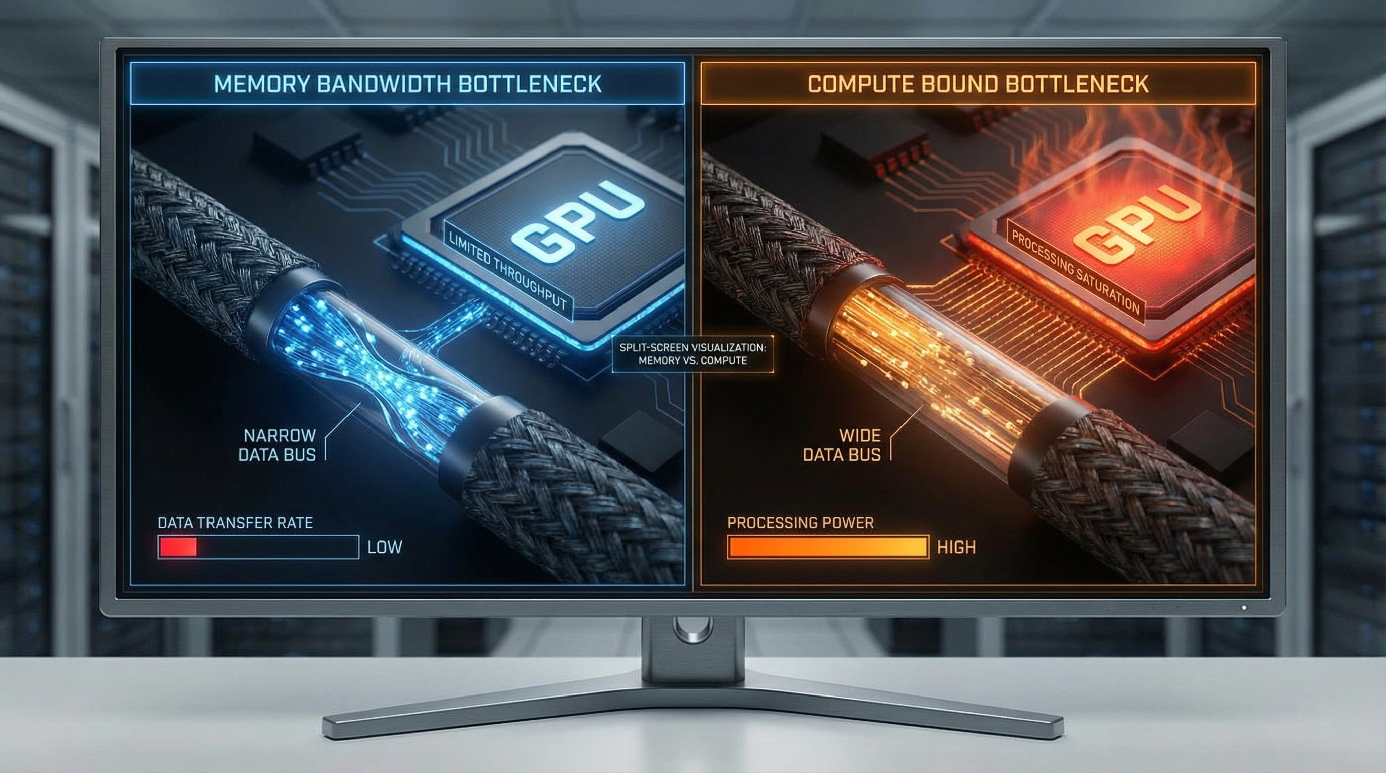
To understand how we run massive models on limited hardware, we must look at the bottleneck. For modern LLM inference, we are rarely compute-bound (limited by TFLOPS); we are almost exclusively memory-bandwidth bound. The time it takes to move weights from VRAM to the Streaming Multiprocessors (SMs) on the GPU is the dominant latency factor.

The Memory Wall and Information Density

Standard inference uses FP16 (16-bit floating point) or FP32.

FP32: 4 bytes per parameter.
FP16/BF16: 2 bytes per parameter.

For an 8-billion parameter model (Llama 3 8B): $Memory_{FP16} \approx 8 \times 10^9 \times 2 \text{ bytes} \approx 16 \text{ GB}$

This fits on an RTX 4090, but barely scrapes by on a 16GB card once you account for the KV Cache (context memory) and overhead. For the 70B model, you need 140GB. This is where Quantization enters the fray.

Mathematical Formulation of Quantization

Quantization maps a high-precision continuous signal (FP16 weights) to a discrete, lower-precision grid (INT4 or INT8). The goal is to minimize the quantization error—the difference between the original weight matrix $W$ and the quantized matrix $Q$ .

Affine quantization can be described mathematically as:

$Q = \text{clamp}\left(\text{round}\left(\frac{W}{S} + Z\right), 0, 2^b - 1\right)$

Where:

$W$ is the input weight tensor.
$S$ is the scale factor (FP32).
$Z$ is the zero-point (integer).
$b$ is the bit-width (e.g., 4).

The de-quantization (performed during inference right before the matrix multiplication) is:

$\hat{W} = S(Q - Z)$

Why INT4 works: The Normal Float 4 (NF4)

Standard integer quantization assumes a uniform distribution of values. However, the weights of a pre-trained neural network trained with Stochastic Gradient Descent usually follow a Gaussian (Normal) distribution, not a uniform one.

Using linear quantization on a bell curve wastes precision on the tails (where few weights exist) and lacks precision in the center (where most weights exist).

The NF4 (Normal Float 4) data type, introduced in the QLoRA paper, is information-theoretically optimal for normally distributed weights. It maps the quantiles of the normal distribution to the discrete 4-bit bins. This ensures that each bin contains roughly the same number of weight values, maximizing entropy and minimizing the Kullback-Leibler (KL) divergence between the original and quantized distributions.

By utilizing NF4, we can compress the model by 4x (from 16 bits to 4 bits) with negligible degradation in perplexity, effectively solving the memory bandwidth bottleneck.

3. Implementation Deep Dive

We will now implement a production-grade inference pipeline using Python. We will use the bitsandbytes library for 4-bit quantization and accelerate for device mapping.

Prerequisites

Ensure you have the CUDA toolkit installed matching your PyTorch version.

pip install torch transformers accelerate bitsandbytes scipy

Part A: Robust Model Loading with NF4

This script demonstrates how to load Llama 3 8B Instruct onto a GPU with limited VRAM using 4-bit quantization. We utilize Bfloat16 for the compute data type to maintain numerical stability during the matrix multiplication steps.

import torch
from transformers import AutoTokenizer, AutoModelForCausalLM, BitsAndBytesConfig
import os

# Configuration constants
MODEL_ID = "meta-llama/Meta-Llama-3-8B-Instruct"
HF_TOKEN = os.getenv("HF_TOKEN") # Ensure your token is set in env vars

def load_quantized_model():
    """
    Loads the Llama 3 model with NF4 quantization configuration.
    Returns tokenizer and model.
    """
    print(f"Initializing model load for: {MODEL_ID}...")
    
    # 1. Define the Quantization Config (The Physics Engine)
    # We use nf4 (Normal Float 4) for weights, but perform calculation in bfloat16
    # Double quantization reduces the memory footprint of the quantization constants themselves
    bnb_config = BitsAndBytesConfig(
        load_in_4bit=True,
        bnb_4bit_quant_type="nf4",
        bnb_4bit_compute_dtype=torch.bfloat16,
        bnb_4bit_use_double_quant=True,
    )

    try:
        # 2. Load Tokenizer
        tokenizer = AutoTokenizer.from_pretrained(MODEL_ID, token=HF_TOKEN)
        tokenizer.pad_token = tokenizer.eos_token # Fix for padding issues
        
        # 3. Load Model with device mapping
        # device_map="auto" will distribute layers to CPU if GPU VRAM is full (offloading)
        model = AutoModelForCausalLM.from_pretrained(
            MODEL_ID,
            quantization_config=bnb_config,
            device_map="auto",
            token=HF_TOKEN,
            low_cpu_mem_usage=True
        )
        
        print("Model loaded successfully. VRAM footprint minimized.")
        return tokenizer, model
        
    except Exception as e:
        print(f"CRITICAL ERROR during model loading: {str(e)}")
        raise e

if __name__ == "__main__":
    tokenizer, model = load_quantized_model()

Part B: The Inference Engine with Streamer

Simply loading the model isn't enough. We need an efficient generation loop. We will implement a TextIteratorStreamer so we don't have to wait for the entire generation to finish before receiving output—essential for user experience.

import threading
from transformers import TextIteratorStreamer

def generate_response(prompt, model, tokenizer, max_new_tokens=512):
    """
    Generates text using a background thread and a streamer for low-latency feedback.
    """
    
    # 1. Format the prompt according to Llama 3 special tokens
    # <|begin_of_text|><|start_header_id|>user<|end_header_id|>

{content}<|eot_id|>
    messages = [
        {"role": "system", "content": "You are a helpful engineering assistant."},
        {"role": "user", "content": prompt},
    ]
    
    input_ids = tokenizer.apply_chat_template(
        messages, 
        add_generation_prompt=True, 
        return_tensors="pt"
    ).to(model.device)

    # 2. Initialize Streamer
    streamer = TextIteratorStreamer(tokenizer, timeout=10.0, skip_prompt=True, skip_special_tokens=True)

    # 3. Define Generation Config
    generate_kwargs = dict(
        input_ids=input_ids,
        streamer=streamer,
        max_new_tokens=max_new_tokens,
        do_sample=True,
        temperature=0.7,
        top_p=0.9,
        eos_token_id=tokenizer.eos_token_id,
    )

    # 4. Run Generation in a separate thread to unblock the main thread for streaming
    t = threading.Thread(target=model.generate, kwargs=generate_kwargs)
    t.start()

    # 5. Yield tokens as they are calculated
    print("
--- Generating Response ---
")
    generated_text = ""
    for new_text in streamer:
        generated_text += new_text
        print(new_text, end="", flush=True)
    
    return generated_text

# Example Usage
# prompt_text = "Explain the difference between laminar and turbulent flow."
# response = generate_response(prompt_text, model, tokenizer)

Part C: Memory Management & Garbage Collection

In a persistent Python process (like a Flask or FastAPI server), GPU memory leaks are fatal. PyTorch caches memory aggressively. You must manually clear the cache between large inference jobs.

import gc

def flush_memory():
    """
    Aggressively reclaims GPU memory.
    Essential for running multiple distinct tasks or handling OOM errors.
    """
    gc.collect()
    torch.cuda.empty_cache()
    if torch.cuda.is_available():
        # Reports current usage for debugging
        print(f"GPU Memory Allocated: {torch.cuda.memory_allocated() / 1024**3:.2f} GB")
        print(f"GPU Memory Reserved:  {torch.cuda.memory_reserved() / 1024**3:.2f} GB")

# Call this after a heavy inference cycle
flush_memory()

4. Advanced Techniques & Optimization

Once the pipeline is running, optimization separates the hobbyists from the engineers.

KV Cache Quantization

While we quantized the weights to 4-bit, the KV Cache (Key-Value cache) grows linearly with context length. For long-context tasks (RAG or document summarization), the KV cache can consume more VRAM than the model weights.

Technique: Use PagedAttention (via vLLM) or 8-bit KV caching. By quantizing the stored activation keys and values, you can double your context window effectively. This introduces a slight noise in the attention mechanism but is generally robust for retrieval tasks.

Speculative Decoding

If you have a powerful GPU but are bound by the serial nature of autoregressive generation (generating one token at a time), use Speculative Decoding.

Load a tiny model (e.g., Llama-3-8B) alongside a massive model (e.g., Llama-3-70B-Int4). The tiny model "drafts" 5-6 tokens rapidly. The large model then performs a single forward pass to verify all draft tokens in parallel. If the large model agrees, you generated 5 tokens in the time of 1. If it disagrees, you roll back. This exploits the fact that memory bandwidth is the bottleneck, but arithmetic intensity (compute) usually has headroom.

Flash Attention 2

Ensure your implementation utilizes Flash Attention 2. Standard attention is quadratic $O(N^2)$ with respect to sequence length. Flash Attention uses IO-awareness to tile the computation, keeping attention scores in high-speed SRAM (L1/L2 cache) rather than swapping to HBM (High Bandwidth Memory). This results in linear scaling in practice and massive speedups for sequences $>2048$ tokens.

Pitfall: Flash Attention requires specific CUDA architectures (Ampere or newer, RTX 30-series+). Ensure you explicitly install the flash-attn pip package compiled for your specific CUDA version, or it will silently fallback to the slow implementation.

5. Real-World Applications

When should you actually use this local implementation over an API?

1. High-Compliance Code Analysis: Large financial institutions and defense contractors often forbid pasting code into ChatGPT. A local Llama 3 instance acting as a coding copilot inside VS Code (using extensions like Continue.dev pointing to your local endpoint) ensures that proprietary algorithms never leave the local subnet.

2. Edge Robotics (The Jetson Use Case): Consider a warehouse robot powered by an NVIDIA Jetson Orin. It needs to interpret natural language commands ("Go pick up the red box near the conveyor"). Cloud latency causes the robot to stutter; WiFi dead zones cause failure. A quantized 8B model running locally allows for fully autonomous semantic processing without internet connectivity.

3. Private RAG (Retrieval Augmented Generation): Law firms dealing with discovery documents can index terabytes of PDFs locally. By running both the embedding model and the generation model (Llama 3) on an on-premise workstation, they can query specific case precedents without uploading client privilege data to a cloud vector database.

6. External Reference & Video Content

In the broader context of the "Local LLM" movement, the video "Running LLMs Locally" serves as a vital primer for the democratization of AI hardware.

The video typically highlights the paradigm shift from "AI as a Service" (SaaS) to "AI as Infrastructure." It underscores the economic argument: while the upfront cost of an RTX 4090 is high ($1,600+), the inference cost is effectively zero (electricity), compared to the recurring, scalable costs of GPT-4 API tokens.

Key takeaways from such educational content often align with our technical implementation:

Privacy is the killer feature: Local execution is the only way to guarantee 0% data leakage.
Quantization is not compression; it's optimization: Understanding that removing precision from noise (tail ends of weight distributions) does not equate to losing intelligence.
The ecosystem is maturing: Tools like llama.cpp, Ollama, and LM Studio are wrapping the complex Python code we wrote above into user-friendly executables, though understanding the Python underbelly is necessary for custom engineering integration.

7. Conclusion & Next Steps

Running Llama 3 on consumer hardware is a triumph of software engineering over hardware limitations. By leveraging the physics of Normal Float 4 quantization and the efficient memory management of modern libraries, we can fit state-of-the-art intelligence into a consumer GPU.

We have covered:

The theoretical bounds of memory bandwidth.
The mathematics of affine quantization.
A complete Python implementation using bitsandbytes.
Advanced optimization strategies like Speculative Decoding.

Next Steps for the Engineer:

Experiment with Fine-Tuning: Now that you can run the model, look into QLoRA to fine-tune it on your specific dataset using the same 4-bit loading techniques.
Explore vLLM: For high-throughput serving (if you are building a local API for a team), migrate from Hugging Face pipelines to vLLM for production-grade concurrent request handling.
Hardware Upgrades: If you are serious about 70B models, consider dual RTX 3090 setups connected via NVLink (if available) or simply PCIe, utilizing tensor parallelism to split the model across cards.

The future of AI isn't just in the cloud; it's on the edge, optimized, private, and under your control.