The Physics of AI: Why Gradient Descent Resembles Energy Minimization

1. Introduction: The Universal Quest for Equilibrium

Imagine you are a condensed matter physicist trying to design a new metallic glass. You are searching for a specific atomic configuration where the material is stable, strong, and resistant to corrosion. In physical terms, you are hunting for the ground state—the configuration of atoms that possesses the lowest possible potential energy.

However, nature is not kind. The energy landscape of this material is rugged, filled with billions of local minima—"metastable" states where the atoms settle comfortably, but not optimally. To find the true ground state, you would traditionally rely on thermal fluctuations (heat) to jiggle the atoms out of these local traps, allowing them to explore the landscape until they cool into the perfect structure. This is the physics of annealing.

Now, switch hats. You are a Machine Learning Engineer training a Deep Neural Network (DNN) with billions of parameters. You are trying to minimize a Loss Function (error). You find that your model gets stuck in suboptimal performance states, unable to generalize.

Here is the revelation: These two problems are mathematically identical.

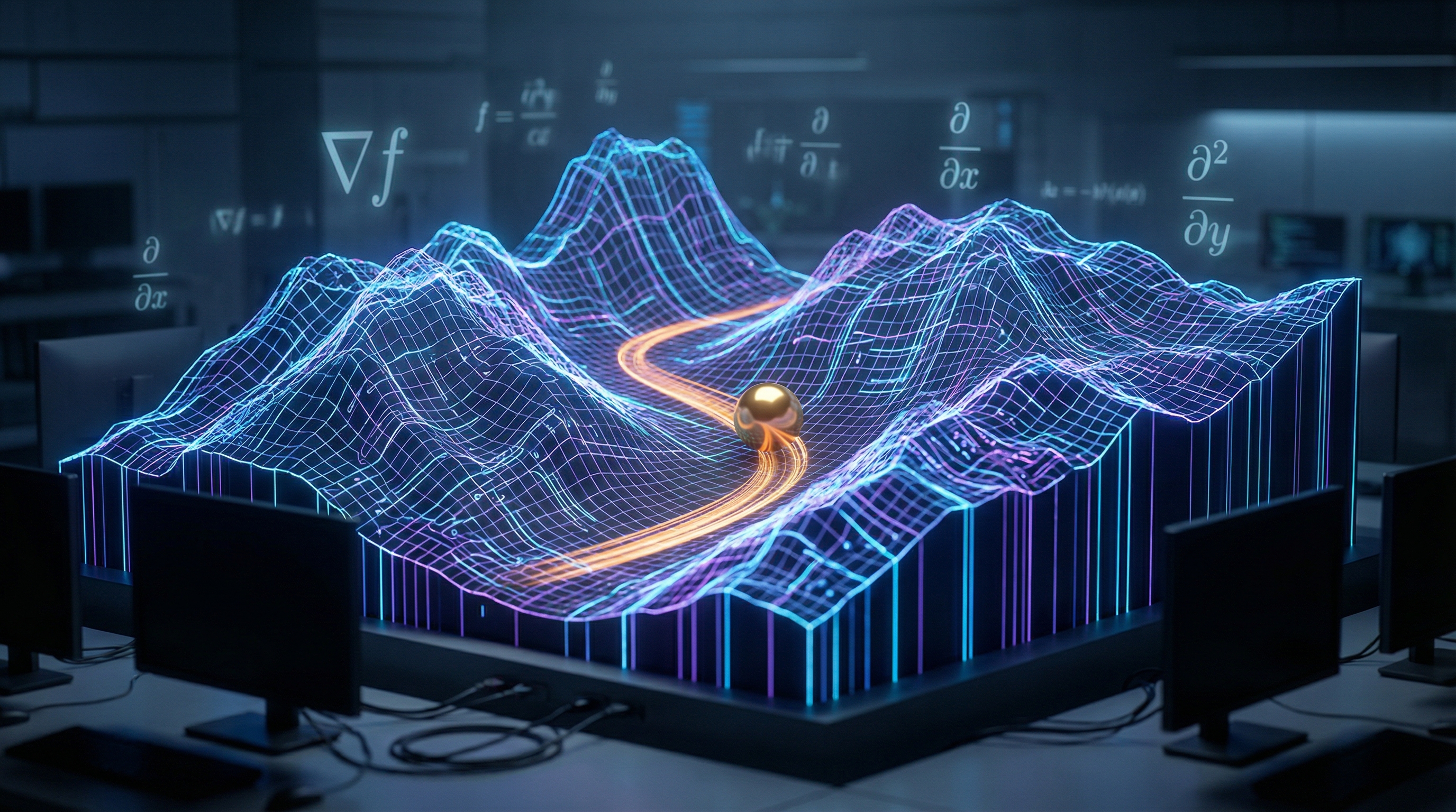
When we train AI, we are not simply "teaching" a computer; we are simulating a physical system relaxing into a low-energy state. The parameters of the network are coordinates in a high-dimensional space, and the loss function is the potential energy surface. Understanding this isomorphism—the mapping between Gradient Descent and Energy Minimization—is not just an academic curiosity. It is the key to unlocking advanced optimization techniques, understanding why Deep Learning works despite the curse of dimensionality, and developing the next generation of algorithms.

In this comprehensive analysis, we will deconstruct the physics of AI, moving from the Hamiltonian mechanics of optimization to implementation in Python, and finally to real-world applications where code meets the laws of thermodynamics.

2. Theoretical Foundation: From Potentials to Gradients

To understand why Gradient Descent works, we must look at it through the lens of classical mechanics and statistical physics.

The Potential Energy Surface (PES)

In physics, a conservative force field $\vec{F}$ is defined as the negative gradient of a potential energy field $U(\vec{x})$ :

abla U(\vec{x}) $$ In Machine Learning, we define a Loss Function $L(\vec{\theta})$, where $\vec{\theta}$ represents the vector of all weights and biases in the network. The goal of the network is to find $\vec{\theta}^*$ such that $L$ is minimized. The update rule for standard Gradient Descent is: $$ \vec{\theta}_{t+1} = \vec{\theta}_t - \eta abla L(\vec{\theta}_t) $$ Where $\eta$ is the learning rate. Notice the similarity? The term $- abla L$ is literally a **force** vector pushing the system parameters "downhill" toward a state of lower energy (lower error). ### Overdamped Dynamics However, there is a nuance. In Newtonian mechanics, $F=ma$. Objects possess inertia. If you drop a ball in a bowl, it doesn't just slide to the bottom and stop; it accelerates, passes the minimum, and oscillates. Standard Gradient Descent actually corresponds to **Aristotelian motion** or **overdamped dynamics** in a highly viscous fluid, where velocity is proportional to force ($v \propto F$), not acceleration. We assume the "friction" is so high that inertia is negligible. ### The Role of Temperature (Stochastic Gradient Descent) In reality, we rarely compute the gradient over the entire dataset (the true energy landscape). We use mini-batches. This introduces noise into the gradient estimation.

abla L_{batch} \approx abla L_{true} + \text{Noise} $$

In physics, this is described by Langevin Dynamics, which models the motion of particles in a fluid subjected to random molecular collisions (Brownian motion).

abla L(\vec{\theta}) dt + \sqrt{2T} dW $$ Here, the "noise" from the mini-batch acts exactly like **Temperature ($T$)** in a physical system. This is crucial. Just as thermal energy helps atoms jump out of local minima in a crystal to find the true ground state, the noise in Stochastic Gradient Descent (SGD) helps the neural network escape poor local minima and saddle points. This implies that **batch size** and **learning rate** together define the "thermodynamic temperature" of your training process. --- ## 3. Implementation Deep Dive: Simulating the Landscape

To visualize this, we will write a Python simulation that treats an optimization problem as a physical simulation of a particle on a rugged terrain. We will use the Rastrigin function, a standard performance test for optimization algorithms due to its large number of local minima.

Setup and Prerequisites

We require numpy for vectorization and matplotlib for visualizing the trajectory on the energy surface.

import numpy as np
import matplotlib.pyplot as plt
from matplotlib.colors import LogNorm

# Configuration for reproducibility
np.random.seed(42)

def rastrigin(x, y, A=10):
    """
    The Rastrigin function: A non-convex function used as a performance 
    test problem for optimization algorithms.
    Think of this as a very rugged energy landscape.
    """
    return A * 2 + (x**2 - A * np.cos(2 * np.pi * x)) + (y**2 - A * np.cos(2 * np.pi * y))

def get_gradients(x, y, A=10):
    """
    Analytical derivatives of the Rastrigin function.
    Corresponds to Force = -Gradient.
    """
    dx = 2 * x + A * 2 * np.pi * np.sin(2 * np.pi * x)
    dy = 2 * y + A * 2 * np.pi * np.sin(2 * np.pi * y)
    return np.array([dx, dy])

Implementation 1: Classical Momentum (The Newtonian Approach)

Standard Gradient Descent often gets stuck in local valleys. To solve this, ML practitioners use "Momentum." In physics terms, we are simply re-introducing mass and inertia to our particle, allowing it to plow through small barriers.

class PhysicsOptimizer:
    def __init__(self, learning_rate=0.01, mass=0.9):
        """
        mass: Corresponds to the momentum coefficient (beta) in ML.
        High mass = high inertia.
        """
        self.lr = learning_rate
        self.mass = mass
        self.velocity = np.zeros(2)

    def update(self, params, grads):
        """
        Updates parameters simulating F = ma.
        v_{t+1} = friction * v_t - lr * gradient
        x_{t+1} = x_t + v_{t+1}
        """
        # Velocity update (incorporating inertia)
        self.velocity = (self.mass * self.velocity) - (self.lr * grads)
        
        # Position update
        new_params = params + self.velocity
        return new_params

# Simulation Loop
start_pos = np.array([4.5, 4.5]) # Starting high on the hill
optimizer = PhysicsOptimizer(learning_rate=0.001, mass=0.9)

trajectory = [start_pos]
current_pos = start_pos

for _ in range(100): grads = get_gradients(current_pos[0], current_pos[1]) current_pos = optimizer.update(current_pos, grads) trajectory.append(current_pos)

trajectory = np.array(trajectory) print(f"Final Position: {current_pos}")


### Implementation 2: Langevin Dynamics (Adding Thermal Noise)

Here we implement **Stochastic Gradient Langevin Dynamics (SGLD)**. We inject Gaussian noise into the gradient step. This effectively gives the particle "thermal energy" to jump out of shallow basins of attraction.

```python
def langevin_update(params, grads, lr, temperature):
    """
    Simulates a particle in a thermal bath.
    temperature: Controls the variance of the injected noise.
    """
    noise_scale = np.sqrt(2 * temperature * lr)
    thermal_noise = np.random.normal(0, noise_scale, size=params.shape)
    
    # The update combines the deterministic force (gradient) 
    # and the stochastic force (thermal noise)
    new_params = params - (lr * grads) + thermal_noise
    return new_params

# Running the Langevin Simulation
thermal_pos = np.array([4.5, 4.5])
thermal_traj = [thermal_pos]

# We use a cooling schedule (Simulated Annealing)
initial_temp = 5.0

for t in range(200):
    # Cooling schedule: Temperature decays over time
    current_temp = initial_temp / (1 + 0.1 * t)
    
    grads = get_gradients(thermal_pos[0], thermal_pos[1])
    thermal_pos = langevin_update(thermal_pos, grads, lr=0.001, temperature=current_temp)
    thermal_traj.append(thermal_pos)

thermal_traj = np.array(thermal_traj)

Comparison and Insights

If you plot these trajectories, you will observe distinct behaviors:

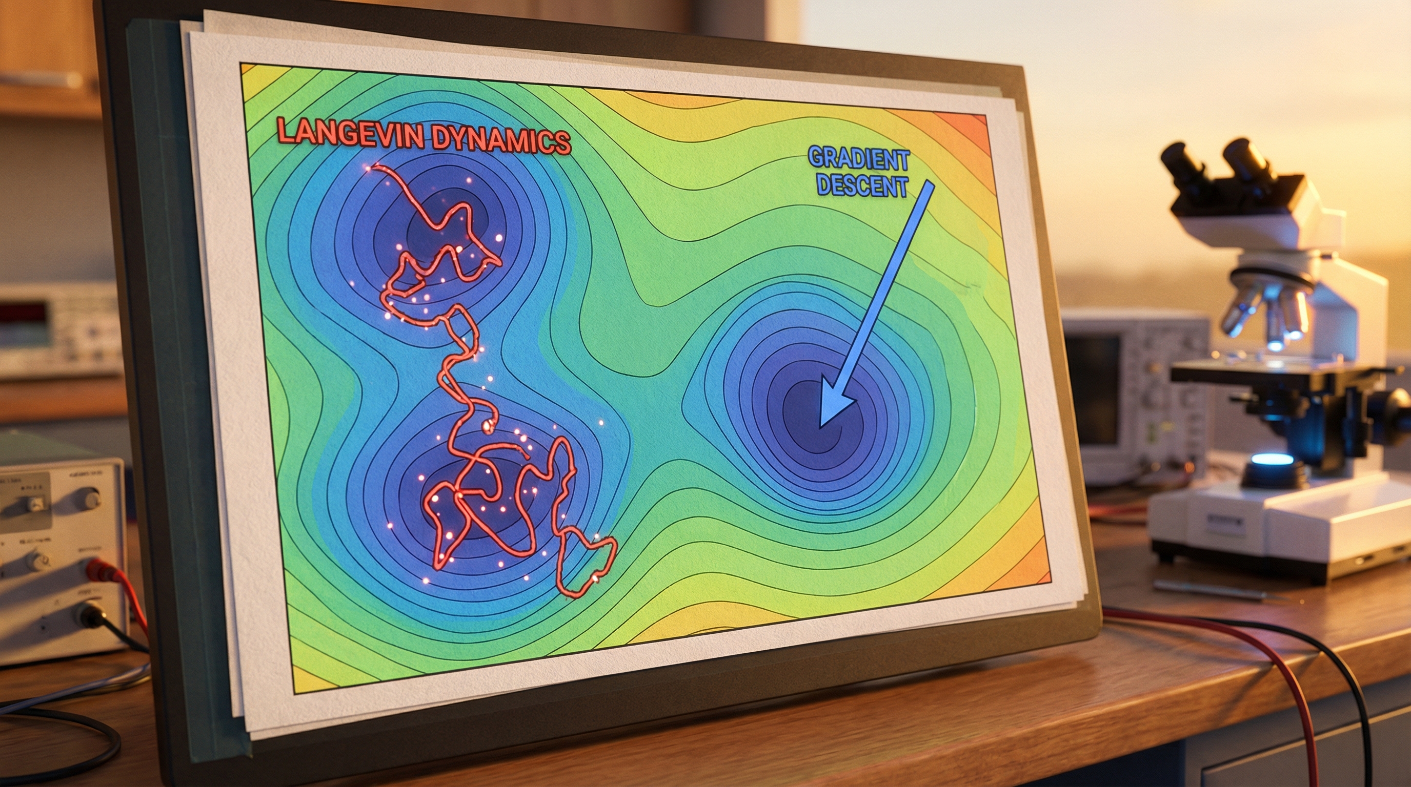
Gradient Descent (Overdamped): Slides directly to the nearest local minimum and stops. It gets stuck easily.
Momentum (Newtonian): Orbits the minima, overshoots, and spirals down. It can cross flat plateaus faster because it builds up speed.
Langevin (Thermodynamic): It behaves erratically. It jumps around local minima. However, as the temperature cools (simulated annealing), it settles. Statistically, it has a higher probability of finding the global minimum because it explores the state space more thoroughly before freezing.

4. Advanced Techniques: Escaping Saddle Points and Curvature

The physics analogy extends beyond simple mechanics into geometry and relativity.

The Curse of Dimensionality and Saddle Points

In 1D or 2D functions (like the Rastrigin above), local minima are the primary enemy. However, in high-dimensional spaces (like a Neural Network with $10^9$ parameters), local minima are mathematically rare. The real enemy is the Saddle Point—a point where the gradient is zero, but the surface curves up in some directions and down in others.

Imagine a horse saddle. If you put a ball in the middle, it is stable left-to-right, but unstable front-to-back.

In high-dimensional physics, we analyze this using the Hessian Matrix (the matrix of second derivatives, describing curvature). For a point to be a true local minimum, all eigenvalues of the Hessian must be positive. In high dimensions, the probability of all eigenvalues being positive by chance is exponentially small.

Physics-Based Solution: Noise (Temperature) helps escape saddle points. Since a saddle point is unstable in at least one direction, any thermal fluctuation along that eigenvector will cause the parameter to "roll off" the saddle, continuing the optimization. This is why SGD often generalizes better than full-batch gradient descent—the noise is a feature, not a bug.

Adaptive Metric Tensors (Adam as General Relativity)

Standard Gradient Descent assumes the geometry of the parameter space is Euclidean (flat). However, the loss landscape often varies wildly in curvature—some directions are steep canyons, others are flat plains.

Advanced optimizers like Adam or RMSprop can be viewed through the lens of Riemannian Geometry. They essentially estimate the local curvature (using the second moment of gradients as a proxy for the diagonal of the Hessian) and adapt the "metric tensor" of the space.

In physics terms, Adam normalizes the friction coefficient for every dimension individually. If a dimension is steep (high force), Adam increases friction (lowers step size) to prevent instability. If a dimension is flat, it decreases friction (increases step size) to accelerate movement. It effectively flattens the energy landscape, turning a rugged canyon into a smooth bowl.

5. Real-World Applications

Understanding optimization as energy minimization transforms how we approach engineering problems across industries.

1. Protein Folding (AlphaFold)

This is the most direct application. A protein's 3D structure is determined by its amino acid sequence settling into the lowest possible free energy state. AlphaFold uses Deep Learning to predict this structure. The training process essentially learns the complex Hamiltonian (energy function) of molecular interactions. By minimizing the loss, the network learns to simulate the physical energy minimization that occurs in nature.

2. Material Science: Crystal Structure Prediction

Engineers designing new battery materials or solar cells need to know how atoms will arrange themselves. This is a Global Optimization problem on a Potential Energy Surface. Techniques like Basin Hopping (a mix of Monte Carlo and Gradient Descent) are standard here. AI models are now trained to act as "surrogate models"—approximating the Quantum Mechanical forces (DFT) to speed up this minimization by orders of magnitude.

3. Chip Floorplanning

Placing billions of transistors on a CPU to minimize heat and latency is an optimization problem analogous to minimizing the tension in a network of springs. The "energy" here is a weighted sum of wire length, thermal density, and signal delay. Annealing algorithms, directly derived from statistical mechanics, are the industry standard for Very Large Scale Integration (VLSI) design.

6. External Reference: The Physics of Machine Learning

For those interested in a deeper theoretical dive, the video "Physics of Machine Learning" provides an excellent visual conceptualization of these topics. It bridges the gap between the Hopfield Network (an early form of RNN) and the Ising Model in magnetism.

The key takeaway from this field of study is that neural networks are not just arbitrary calculators; they are dynamic systems that obey statistical laws. The "training" phase is a trajectory through a thermodynamic state space. When a network "overfits," it is analogous to a system getting stuck in a "glassy" state—frozen in a local configuration that doesn't represent the true nature of the data. Regularization techniques (like Dropout or Weight Decay) act as entropy terms, forcing the system to remain simpler and more robust, much like preventing a metal from becoming too brittle.

7. Conclusion: The Grand Unification

The convergence of Physics and AI is one of the most exciting developments in modern science. We have learned that:

Gradient Descent is not just math; it is the simulation of a particle moving through a viscous medium under the influence of a potential force.
Momentum and Adam are modifications to the physical laws of that universe (adding inertia or warping geometry) to facilitate faster convergence.
Noise (SGD) is equivalent to Temperature, preventing the system from freezing into suboptimal metastable states.

For the engineer, this perspective shifts the mindset from "tuning hyperparameters" to "designing the dynamics of the system." If your model is unstable, your "friction" (learning rate) might be too low. If it's stuck, your "temperature" (batch noise) might be too cold.

Next Steps:

Experiment with the provided Python code by changing the mass and temperature variables to see how the trajectory changes.
Read up on Hamiltonian Monte Carlo (HMC), a powerful sampling method that uses conservation of energy to explore probability distributions.
Explore JAX, a library that treats Python code as differentiable math, making physics-based optimization incredibly efficient.

By treating AI as a physical system, we stop guessing and start engineering with the fundamental laws of nature.