Using Python for Spectral Analysis of Material Properties

1. Introduction: The Signal in the Noise

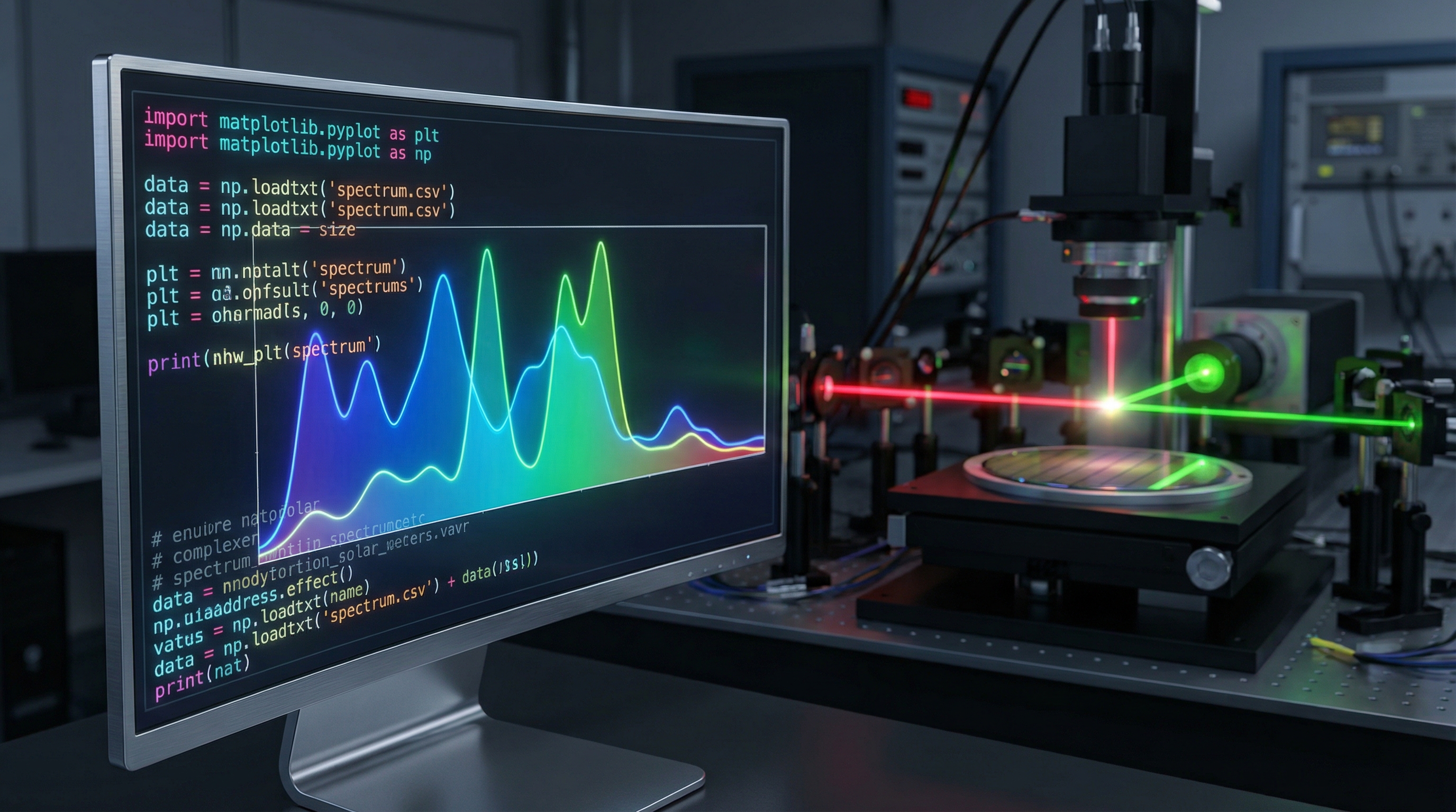
Imagine you are a process engineer at a semiconductor fabrication plant. A multimillion-dollar batch of silicon wafers has just failed electrical testing. The electron microscopy looks standard, but the electrical conductivity is off by an order of magnitude. You suspect a contaminant—perhaps a trace amount of organic residue from a cleaning step, or a subtle stoichiometric imbalance in the thin-film deposition. You turn to Raman spectroscopy or Fourier Transform Infrared (FTIR) spectroscopy.

The instrument spits out a jagged line: a spectrum. To the untrained eye, it is a mess of static and bumps. To the proprietary software that came with the machine, it might be "Unknown Material." But to a physicist armed with Python, that noisy signal is a fingerprint. It contains the vibrational eigenmodes of the crystal lattice, the rotational energy levels of the contaminant molecules, and the tell-tale scattering cross-sections that reveal the material's soul.

Reliance on closed-source, vendor-specific software is the bottleneck of modern materials science. It obfuscates the underlying physics, limits your ability to customize background subtraction, and often fails when signal-to-noise ratios (SNR) drop below comfortable thresholds. By migrating your spectral analysis workflow to Python, you gain control. You gain the ability to batch-process thousands of spectra, apply rigorous statistical noise reduction without destroying data, and mathematically deconvolve overlapping peaks to identify hidden phases.

In this post, we will bypass the GUI buttons and write the code that connects the quantum mechanical nature of light-matter interaction directly to actionable engineering data. We will move from raw CSV files to precise quantitative analysis of material properties, building a pipeline that is robust, reproducible, and scientifically rigorous.

2. Theoretical Foundation: Physics and Fourier

To analyze a spectrum effectively, we must first understand what the data represents mathematically and physically. In spectroscopy (whether Raman, FTIR, or X-ray Photoelectron Spectroscopy), we are essentially measuring the interaction of an electromagnetic field with matter.

The Physics of Lineshapes

At the quantum level, transitions between energy states (electronic, vibrational, or rotational) are not infinitely sharp. According to the Heisenberg Uncertainty Principle ( $\Delta E \Delta t \ge \hbar/2$ ), the finite lifetime of an excited state results in a broadening of the spectral line.

Ideally, a spectral peak is modeled by a Lorentzian function, which describes the homogeneous broadening caused by the natural lifetime of the state:

$L(x; x_0, \gamma) = \frac{1}{\pi} \left[ \frac{\gamma}{(x - x_0)^2 + \gamma^2} \right]$

Where $x_0$ is the peak position (energy/wavenumber) and $\gamma$ is the half-width at half-maximum (HWHM). However, in real-world experimentation, instrumental artifacts (diffraction limits, slit widths) and inhomogeneous broadening (thermal Doppler effects, local disorder) introduce a Gaussian component.

Therefore, the most accurate mathematical model for a spectral peak in material analysis is the Voigt Profile, which is a convolution of a Lorentzian and a Gaussian profile:

$V(x; \sigma, \gamma) = \int_{-\infty}^{\infty} G(x'; \sigma) L(x - x'; \gamma) dx'$

Understanding this is critical because the Gaussian width often correlates to instrumental resolution or temperature, while the Lorentzian width correlates to the material's crystalline quality or phonon lifetime. A naive analysis using simple peak-finding algorithms without fitting these profiles will yield inaccurate material properties.

The Mathematics of Signal Processing

Before we can fit peaks, we often deal with background noise and fluorescence. Fluorescence acts as a broad, low-frequency continuum added to our high-frequency spectral peaks. Mathematically, the observed signal $S_{obs}$ is:

u) = S_{peaks}( u) + B_{fluorescence}( u) + N_{noise} $$ Our coding logic must perform two distinct operations: 1. **Low-pass filtering** (or polynomial subtraction) to remove $ B_{fluorescence} $ without distorting peak shapes. 2. **Smoothing** to reduce $ N_{noise} $, typically utilizing a Savitzky-Golay filter. This filter effectively fits a local polynomial to a window of points and replaces the center point with the polynomial's value, preserving the moments of the distribution better than a standard moving average. --- ## 3. Implementation Deep Dive Let's construct a robust Python pipeline for spectral analysis. We will rely on `numpy` for array manipulation, `scipy` for signal processing, and `lmfit` for non-linear least-squares minimization, which is superior to `scipy.optimize` for constraining physical parameters. ### Prerequisite Libraries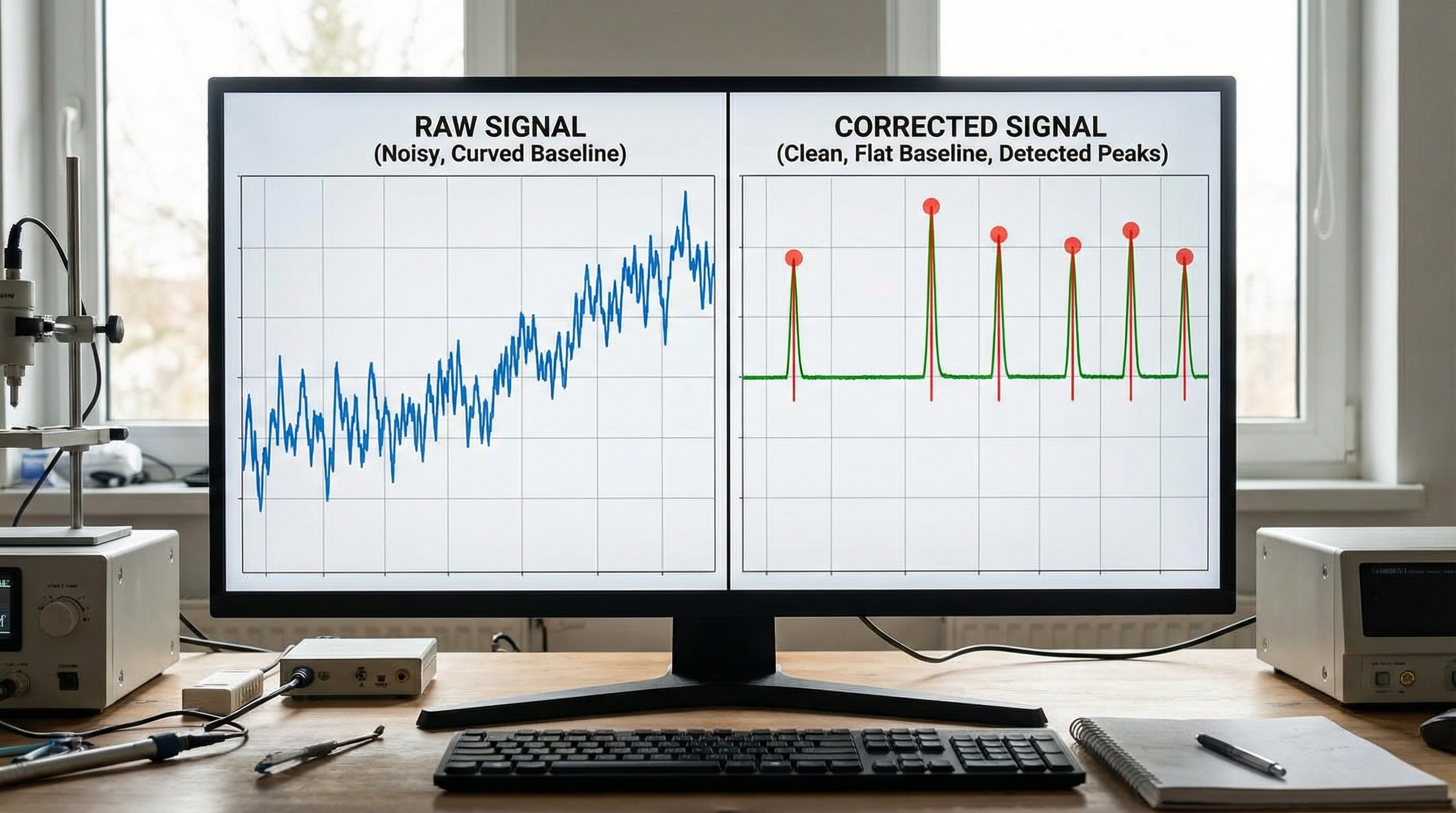

import numpy as np
import matplotlib.pyplot as plt
from scipy.signal import savgol_filter, find_peaks
from scipy import sparse
from scipy.sparse.linalg import spsolve
import lmfit
from lmfit.models import VoigtModel, ConstantModel

# Ensure reproducibility
np.random.seed(42)

Step 1: Generating Synthetic Data (for demonstration)

In a real scenario, you would load data via pandas.read_csv. Here, we simulate a noisy Raman spectrum with a fluorescent background.

def generate_mock_spectrum(x):
    # Simulate three distinct material peaks (Voigt profiles)
    p1 = 10.0 * np.exp(-0.5 * ((x - 800) / 10)**2)  # Gaussian approximation for simplicity here
    p2 = 15.0 * np.exp(-0.5 * ((x - 1050) / 15)**2)
    p3 = 5.0 * np.exp(-0.5 * ((x - 1100) / 8)**2)
    
    # Add a broad fluorescent background (simulated as a polynomial/exponential)
    background = 50 + 0.05 * x + 0.0001 * x**2 + 20 * np.sin(x / 500)
    
    # Add random detector noise
    noise = np.random.normal(0, 1.5, size=len(x))
    
    return p1 + p2 + p3 + background + noise

wavenumbers = np.linspace(400, 1800, 2000)
intensity = generate_mock_spectrum(wavenumbers)

plt.figure(figsize=(10, 6))
plt.plot(wavenumbers, intensity, color='black', alpha=0.7, label='Raw Data')
plt.title("Raw Spectroscopic Data with Fluorescence & Noise")
plt.xlabel("Wavenumber (cm$^{-1}$)")
plt.ylabel("Intensity (a.u.)")
plt.legend()
plt.show()

Step 2: Advanced Baseline Correction (Asymmetric Least Squares)

Simple polynomial fitting often fails because it requires user guessing. The Asymmetric Least Squares (ALS) smoothing is the gold standard in spectroscopy. It iteratively fits a baseline that tries to stay under the data peaks.

def baseline_als(y, lam, p, niter=10):
    """
    Asymmetric Least Squares Baseline Correction.
    
    Parameters:
    y : array_like - The spectral intensity data
    lam : float - Smoothness parameter (usually 10^2 to 10^9)
    p : float - Asymmetry parameter (0.001 to 0.1)
    """
    L = len(y)
    D = sparse.csc_matrix(np.diff(np.eye(L), 2))
    w = np.ones(L)
    for i in range(niter):
        W = sparse.spdiags(w, 0, L, L)
        Z = W + lam * D.dot(D.transpose())
        z = spsolve(Z, w*y)
        w = p * (y > z) + (1-p) * (y < z)
    return z

# Apply correction
baseline = baseline_als(intensity, lam=100000, p=0.001)
corrected_spectrum = intensity - baseline

plt.figure(figsize=(10, 6))
plt.plot(wavenumbers, corrected_spectrum, color='blue', label='Corrected')
plt.plot(wavenumbers, baseline, color='red', linestyle='--', label='Estimated Baseline')
plt.title("Baseline Correction via Asymmetric Least Squares")
plt.legend()
plt.show()

Step 3: Peak Finding and Voigt Fitting

Now that we have a clean spectrum, we need to extract physical parameters. We find initial guesses using find_peaks and then refine them using lmfit.

# 1. Smoothing to assist peak finding (Savitzky-Golay)
# Window length must be odd, polyorder typically 2 or 3
smoothed = savgol_filter(corrected_spectrum, window_length=21, polyorder=3)

# 2. Find peaks (Height threshold depends on SNR)
peaks, properties = find_peaks(smoothed, height=3.0, width=5)
print(f"Found peaks at indices: {peaks}")

# 3. Setup the Composite Model for fitting
model = ConstantModel()
params = model.make_params(c=0)

for i, peak_idx in enumerate(peaks):
    center_guess = wavenumbers[peak_idx]
    height_guess = properties['peak_heights'][i]
    
    # Create a Voigt model for each peak
    prefix = f'p{i}_'
    peak_model = VoigtModel(prefix=prefix)
    
    # Set constraints and guesses
    # Sigma: Gaussian width, Gamma: Lorentzian width
    params.update(peak_model.make_params(
        center=dict(value=center_guess, min=center_guess-10, max=center_guess+10),
        amplitude=dict(value=height_guess*10, min=0),
        sigma=dict(value=5, min=0.1),
        gamma=dict(value=5, min=0.1)
    ))
    
    model += peak_model

# 4. Perform the Fit
result = model.fit(corrected_spectrum, params, x=wavenumbers)

# 5. Visualize Results
plt.figure(figsize=(10, 6))
plt.plot(wavenumbers, corrected_spectrum, 'k.', alpha=0.3, label='Data')
plt.plot(wavenumbers, result.best_fit, 'r-', linewidth=2, label='Best Fit')
plt.title("Multi-Peak Voigt Fitting")
plt.legend()
plt.show()

print(result.fit_report(min_correl=0.5))

Interpretation of the Code

The magic happens in the lmfit loop. We dynamically construct a model based on the number of peaks detected. By constraining sigma and gamma, we ensure the physics remains valid (widths cannot be negative). The result.fit_report provides not just the peak centers, but the errors on those centers. If p1_center has an error of $\pm 0.01$ cm $^{-1}$ , you have high confidence. If the error is $\pm 10$ , your model is overfitting noise.

4. Advanced Techniques & Optimization

Moving beyond basic scripting, elite spectral analysis requires handling edge cases and performance bottlenecks.

Optimization with Vectorization and Numba

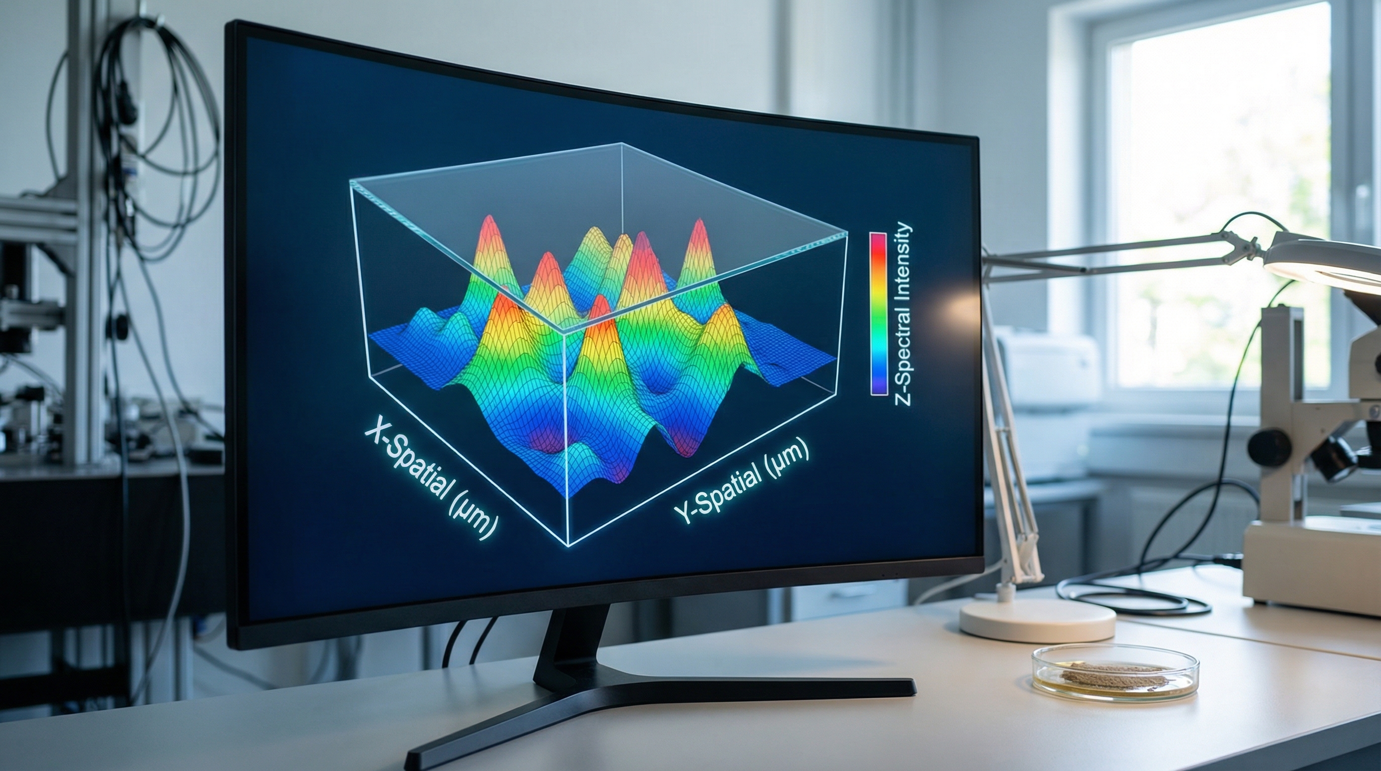
If you are processing hyperspectral images (where every pixel contains a full spectrum), Python loops will kill your performance.

Vectorize operations: Instead of looping through spectra to subtract baselines, structure your data as a 2D matrix (N_samples x M_wavelengths) and use linear algebra operations.
JIT Compilation: For the ALS algorithm, the loop is unavoidable. Use the @jit decorator from numba to compile the function to machine code, providing C++ level speeds.

from numba import jit

@jit(nopython=True)
def fast_als_loop(y, lam, p, niter=10):
    # Numba-optimized implementation details...
    pass

Pitfalls: The "Over-Smoothing" Trap

One common error is aggressive use of the Savitzky-Golay filter. While it produces visually pleasing smooth lines, it broadens peaks and reduces their amplitude. This distorts the calculation of Full Width at Half Maximum (FWHM), which is often used to calculate crystallite size (via the Scherrer equation in XRD) or phonon lifetimes. Always fit on raw or baseline-corrected data, never on heavily smoothed data. Use smoothing only for peak detection logic.

Handling Instrument Response Functions (IRF)

In high-precision physics, the data you collect is the convolution of the true spectrum and the Instrument Response Function. If your spectrometer has a resolution of 4 cm $^{-1}$ , you cannot distinguish features narrower than this. Advanced analysis involves Deconvolution (e.g., Richardson-Lucy algorithm) to remove the IRF, though this is computationally expensive and amplifies noise.

5. Real-World Applications

Where is this code actually used in industry and academia?

1. Strain Analysis in Silicon Microchips

Raman spectroscopy is the industry standard for measuring stress in silicon. The characteristic Silicon peak sits at 520.7 cm $^{-1}$ . Mechanical stress shifts this peak: compressive stress moves it up, tensile stress moves it down. The shift is minute—often less than 0.5 cm $^{-1}$ .

Using the Voigt fitting method above, we can determine the peak center with a precision of 0.02 cm $^{-1}$ , allowing engineers to map stress fields near Through-Silicon Vias (TSVs) that could cause device cracking.

2. Polymorph Identification in Pharmaceuticals

Active Pharmaceutical Ingredients (APIs) can exist in different crystal structures (polymorphs). One form might be therapeutic, another biologically inert or toxic. These polymorphs have distinct spectral signatures in the Terahertz and Raman regions. Python scripts automate the comparison of batch samples against a database of known polymorph spectra, calculating similarity scores (using Cosine Similarity or Euclidean Distance) to flag bad batches instantly.

3. Battery Degradation Analysis

In Lithium-ion battery research, in-operando FTIR is used to monitor the formation of the Solid Electrolyte Interphase (SEI). By tracking the evolution of specific functional group peaks (like C=O or C-O) over time, researchers can quantify decomposition rates. The batch processing capabilities of Python allow for the analysis of gigabytes of time-resolved spectral data that Excel simply cannot handle.

6. External Reference: "Spectral Analysis Techniques"

The video "Spectral Analysis Techniques" serves as an excellent visual companion to the code provided here. While our post focuses on the digital reconstruction of the signal, the video illustrates the analog acquisition pipeline—how diffraction gratings disperse light and how CCD detectors convert photons to electrons.

Crucially, the video touches on the concept of Dynamic Range and Dark Current. In our code, we subtracted a constant or polynomial background. The video explains the physical origin of that background (thermal noise in the detector). Understanding that the "noise" is often Poissonian (shot noise) validates our choice of Least Squares fitting (which assumes Gaussian errors) for high-intensity signals, but suggests that for photon-starved regimes (low light), Maximum Likelihood Estimation (MLE) might be statistically more appropriate. Viewing this content bridges the gap between the hardware settings on your spectrometer and the sigma parameters in your Python script.

7. Conclusion & Next Steps

We have journeyed from the theoretical broadening of quantum states to a fully functional Python pipeline capable of cleaning, detecting, and fitting spectral features. By leveraging the lmfit and scipy ecosystem, you are no longer dependent on "black box" software that hides the nuance of your data.

Key Takeaways:

Physics First: Always model peaks with Voigt profiles to account for both instrument and material effects.
Baseline Matters: Use Asymmetric Least Squares rather than manual subtraction for consistent results.
Fit the Raw Data: Use smoothing for detection, but fit the model to the original data to preserve resolution.

Next Steps: To further elevate your analysis, investigate Chemometrics. Techniques like Principal Component Analysis (PCA) and Partial Least Squares (PLS) Regression allow you to analyze the entire spectrum at once, identifying correlations in complex mixtures that single-peak fitting might miss. Python's scikit-learn library makes this transition seamless.

The data is there. You just need the right code to make it speak.